MISC 006: a proxy measure of the audio stimuli

Important

This example requires the meg_wiki package to download the sample dataset. This package can be installed with pip:

$ pip install git+https://github.com/fcbg-platforms/meg-wiki

The Crimson 3 audio interface has 2 monitoring feedback outputs, Phones 1 is connected with a jack to BNC cable to an analogical input of the MEG acquisition system, MISC 006. This measure of the auditory stimuli can be a good proxy for the auditory waveform, depending on the waveform frequency content. The MEG signal will sample the analogical channels simultaneously with the MEG channels, at the same sampling frequency, by default 1 kHz. Thus, any sound that can be sampled at 1 kHz will be available in the FIF file.

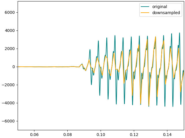
If the auditory stimuli can not be sampled at 1 kHz, this measure can still be a good proxy to check the waveform, its onset and offset and the delay between the onset and the trigger.

Warning

If the sound can not be sampled at 1 kHz, extra care should be taken to ensure that this proxy measure is representing well-enough the auditory stimuli.

Sentence

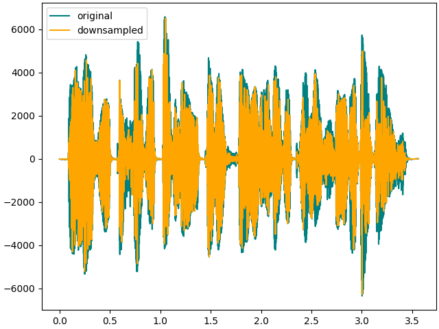
Let’s start by emulating the result of a 1 kHz downsampling on a 24 kHz wav file containing a sentence generated with the text-to-speech tool Amazon Polly.

import numpy as np
from matplotlib import pyplot as plt
from scipy.io import wavfile

from meg_wiki.datasets import sample

fname = sample.data_path() / "tutorials" / "sentence.wav"
fs, data = wavfile.read(fname)
times = np.arange(len(data)) / fs
step = int(fs / 1000)  # step to downsampling to 1 kHz

f, ax = plt.subplots(1, 1, layout="constrained")
ax.plot(times, data, color="teal", label="original")
ax.plot(times[::step], data[::step], color="orange", label="downsampled")
ax.legend()
plt.show()

In this case, the downsampled signal is a good proxy for the original signal. Importantly, the onset is preserved.

f, ax = plt.subplots(1, 1, layout="constrained")
ax.plot(times, data, color="teal", label="original")
ax.plot(times[::step], data[::step], color="orange", label="downsampled")
ax.legend()
ax.set_xlim(0.05, 0.15)
plt.show()

Pure tone

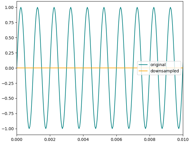
Let’s now consider a pure tone at a badly chosen 1 kHz frequency, exacerbing a badly sampled signal at a sampling frequency of 1 kHz.

data = np.sin(2 * np.pi * 1000 * times)
f, ax = plt.subplots(1, 1, layout="constrained")
ax.plot(times, data, color="teal", label="original")
ax.plot(times[::step], data[::step], color="orange", label="downsampled")
ax.legend()
ax.set_xlim(0, 0.01)
plt.show()

Estimated memory usage: 215 MB